About the Sensory Island Task (SIT)
This blog post is about SIT, a behavioral paradigm we recently published (Ferreiro et al., 2020). In SIT, animals explore an open-field arena to find a sensory target. For target detection, they rely solely on changes in the presented stimulus. Stimulus presentation is controlled by closed-loop position tracking in real-time.
The general Idea of SIT is to allow the investigation of sensory and cognitive processing under more natural conditions than most other paradigms. Therefore, we modified and expanded previous closed-loop free navigation protocols (e.g. Polley et al., 2004 & Whitton et al., 2014), resulting in our current versions of SIT (Ferreiro et al., 2020). With SIT you can study sensory processing of variable modalities (e.g. sound or light) and cognition (e.g. discrimination learning) in moving and actively engaged animals. It also allows for simultaneous neural recordings, if desired.
About this blog post
Here, I will provide hands-on tips on how to use a Python-based version of SIT to train mouse lemurs (or other small mammals) in an acoustic frequency discrimination task in an open field maze. The Python notebook I used to control my setup during the experiments described in our original publication can be downloaded from Andrey’s GitHub repository. I have since introduced some new features to the notebook, such as an additional timer correcting for an animal’s reaction time. You can find this newer version of the notebook in my GitHub repository as “One_Target_SIT.ipynb”, but be aware of the fact that this is work in progress. You will find detailed instructions on how to install the freeware components necessary for running the notebooks in both repositories, so the installation will not be covered in this blog. Instead, I will guide you step-by-step through a single (acoustic) SIT experiment under the assumption that your setup (both hardware and code) are operational.
If you would like to use SIT but you are currently lacking a high-quality open field maze, make sure to visit my DIY instructions on how to build one.
How does the actual experiment look like?
In the example experiment described in this post, a mouse lemur will be trained in an acoustic discrimination task. The training session will last for a maximum of 60 minutes or 50 completed trials, depending on which of both events is reached first. The trial number is mainly limited by the capacity of your food dispenser and the motivation of your experimental animal. Here we use two self-built dispensers, each of them having space for 27 rewards. Mouse lemurs can be quite lazy and 50 trials in one hour is an ambitious, but realistic goal. In the best case scenario, with the animal finishing 50 trials correctly, the food dispensers would still have two spare rewards, each. Let us briefly go through one of the trials to give you an idea of what I mean when I am writing about “trials”:
An individual trial starts as soon as the experimental animal visits a fix starting area (Fig. 1; magenta circle) for a pre-defined initiation duration. In the example setup, an inverted glass Petri dish was put to the center of the starting area to provide some visual and haptic information on its location.

Figure 1. In this frame, the experimental animal is between two trials as signalled to the experimenter by the big red dot in the upper left corner of the picture. The previous trial was finished and the animal has not yet visited the starting area (magenta circle) to initiate a new trial. The current position of the animal is calculated as the center of the animal’s contour (orange dot).
At the moment of trial initiation, a virtual, circular target area is calculated and randomly positioned within the maze (Fig. 2; yellow circle). In addition, the playback of a short (57 ms), high-pitched (10 kHz) pure tone starts at a repetition frequency of approximately 5 Hz. The playback continues as long as the animal is outside the target area or until the maximum trial duration is reached.
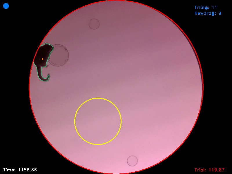
Figure 2. In this frame, the animal has just initiated the trial and is still sitting in the former starting area. It now has to start searching for the hidden target area (yellow circle). The blue dot in the upper left corner of the picture indicates that the trial has started. In the lower right corner a trial timer shows how much time is left for the animal to find the target and to successfully complete the trial.
As soon as the experimental animal enters the target area while exploring the maze, the audio playback switches to a new pure town of the same length, volume, and repetition frequency as the previous tone, but with a different pitch (4 kHz). This shift in pitch from 10 kHz to 4 kHz is the only information the experimental animal can reliably use for target detection. Once found, the animal has to stay within the target for a pre-defined target duration to get a reward (Fig. 3).
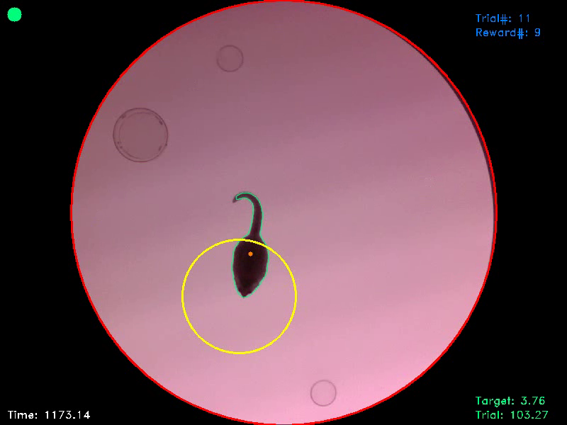
Figure 3. In this frame, the animal entered the target area, as signalled to the experimenter by a green dot in the upper left corner of the picture. At the same time the animal enters the target area, the trial timer freezes and a target timer starts counting backwards. If this target counter reaches zero, as the animal remained within the target for the entire target duration, the trial ist terminated and the animal gets a reward. If the animal leaves the target area before the target duration has passed, the trial timer continues and the target counter resets.
If the animal leaves the target area before the target duration is reached, the playback switches back to the high-pitched (10 kHz) sound and the animal has to re-visit the target for another full target duration and within the trial duration to get a reward. Delivery of a reward after successful completion of the trial or automatic trial termination after the maximum trial duration has passed without the animal being successful stops the audio playback and the animal has to re-visit the starting platform to initiate a new trial with a new target location.
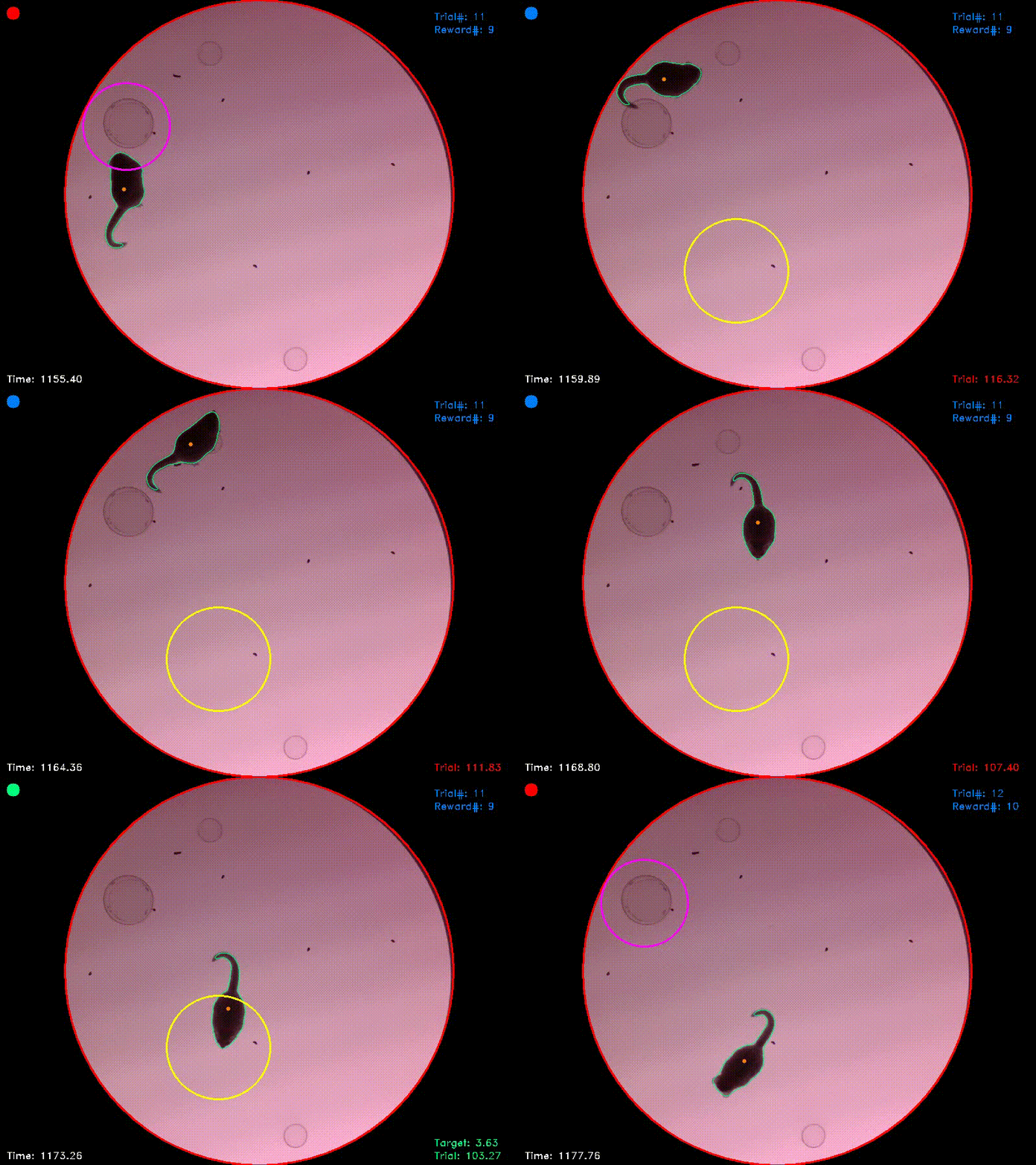
Video 1. This video shows the entire trial from which Figs. 1-3 were captured. It starts shortly before trial initiation and ends shortly after successful trial completion. You can see that at the moment of trial completion, both the trial counter and the reward counter in the upper right corner increment by one.
Preparing the experiment
Before you start with your own experiments, some preparations should be made. First and foremost, it is always a good idea to check if the individual components of your setup are operational. For the acoustic experiment described below, this includes an audio amplifier and a loud speaker (for the acoustic stimulation), a webcam (for the real-time video tracking), two food dispensers, driven by arduinos (for rewarding the animal after successful trials), and the illumination of the maze floor (for contrast enhancement). I usually run the entire notebook and complete a few trials myself to make sure that everything works. You should also check, if there is enough space on your hard drive for saving the video protocol. If space runs out during an ongoing experiment, you will lose important data.
Further preparations include:
- a thorough cleaning of the open field maze with 70% ethanol (to remove any remains and scent marks from previous experiments)
- filling of the food dispensers (it would be unfortunate to run out of rewards during an ongoing session)
- catching of the animal, if necessary, and preparation of its transport to the setup
- placing of free rewards (e.g. in the starting area as initial motivators)
Getting started
The Jupyter Notebook that controls the entire hardware during the experiment has a total of 15 cells, which can be executed either individually or all at once (Fig. 4). For your first experiments, I recommend executing the code cell after cell to get accustomed to the individual steps of the protocol. Once you internalized the procedure and its individual steps, you will probably choose the other option. In any case, I recommend using the “Kernel” dropdown menu to restart the kernel and to clear all previous output of the notebook before starting a new experiment.
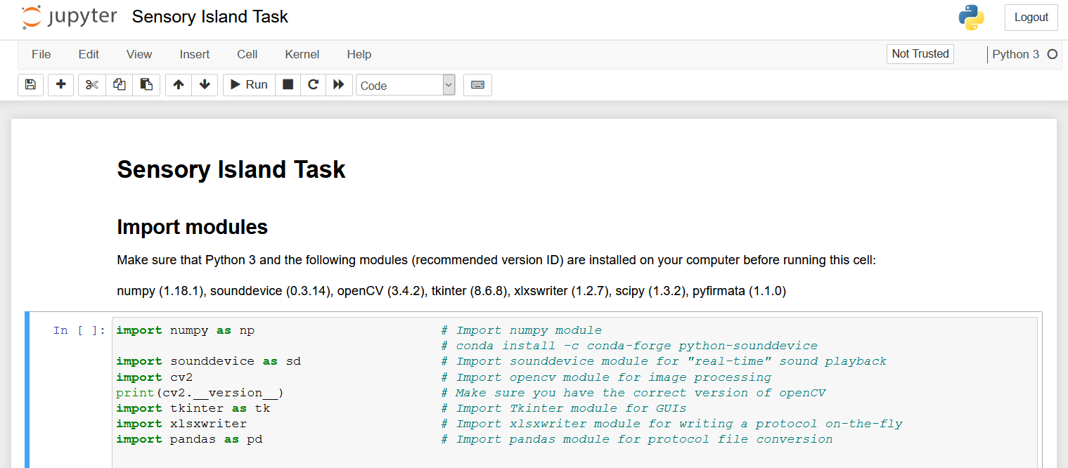
Figure 4. Once you opened the notebook in Jupyter, it should look something like this. You can either select individual cells of code and execute them using the “> Run” button or you can open the “Cell” dropdown menu and select “Run All” to run all the cells at once.
The first two cells can be executed without hesitation. They simply import all the Python modules needed (cell 1) and define some functions (cell 2) that are later used in the main code. In the third cell, you can specify the position and dimension of your arena in the video feed (Fig. 5). Normally, you will not have to change these values once they are set, unless you change your setup. The position of the arena is specified by the XY-coordinates of its center point and the size of the arena is defined by its radius in pixels (which means only circular arenas are supported).

Figure 5. In cell 3 you can specifiy the XY-coordinates and size of your arena in pixels. Normally you should only have to do this once before your very first experiment.
My camera has a resolution of 800x600 pixels and is installed exactly above the center of our maze. The distance between maze floor and camera is chosen in a way that the maze floor fills the entire height of the picture (e.g. Video 1). I recommend a similar calibration for your setup, as it optimally uses the resources. In times of 4K television the video resolution we chose may seem low, but for small setups of below 100 cm in diameter, the resulting spatial resolution totally suffices. Remember that the video tracking is performed in real-time and the more unnecessary pixels your video has, the more computing power you will waste.
Setting the session parameters
Cell 4 is the first cell of the notebook that is really important for the session we are about to start. As soon as you execute this cell, a new window will pop up and ask you to set the parameters for the current experiment (Fig. 6).
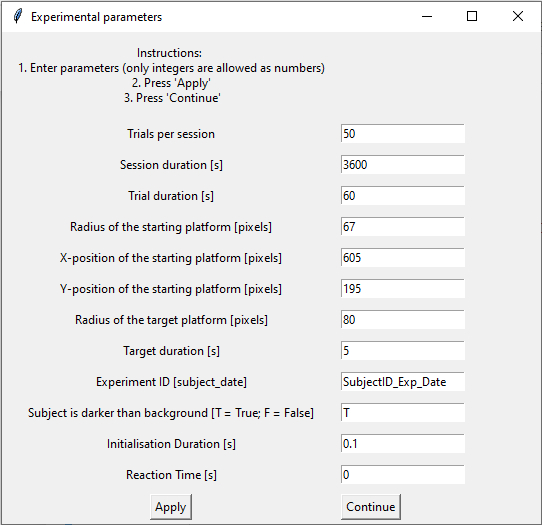
Figure 6. This is the window in which you can enter and set the different parameters for each new session.
Every time the notebook is run, the window starts with some default values for each parameter. If you do not change anything (which I do not recommend, as you should at least give your experiment an identifier), the session will later start using these values. However, you will likely want to change some of the parameters. The number of trials per session and the session duration are the values that define the duration of your experiment, as the session will end as soon as one of these values is reached. The trial duration is the time interval during which the animal has to find the target island after trial initiation.
The radius and the X- and Y-position of the starting platform define the size and location of the area the animal has to visit to initiate each trial (magenta circle in Video 1). In my experiments, the location and size of this starting area never changed, but there may be experiments where such a change in position between sessions is necessary.
The radius of the target platform specifies the size of the target island (yellow circle in Video 1) the animal has to find. Remember that the location of the target changes randomly on a trial-to-trial basis. Therefore, you cannot enter XY-coordinates for the target. The target duration is the time the animal has to stay within the target area to successfully finish a given trial and to get a reward. The smaller the target area and the longer the target duration, the more difficult it is for the animal to complete the trial successfully. If your animal is naive to the task, you will probably start with a large target and short target duration. However, you have to keep in mind that the larger the target is and the shorter the target duration are, the less clear it is if the animal’s behavior during a successful trial is a real response to the changing stimulus or an accidental stop within the target area. You will have to use small targets and long target durations at some point to be able to distinguish those accidental stops, which frequently occur during normal exploration, from intended stops (see Ferreiro et al., 2020 for helpful statistics).
The experiment ID is used to later identify your experiment. All protocols generated by the script (a text file listing the session parameters, a video of the experiment, and a .xlsx as well as a .csv file with positional data from each frame) will automatically have this ID in their file name. This said, make sure to choose a unique ID for each experiment or you will lose data, as previous files with the same name will be overwritten. I would recommend using the following, unambiguous format: SubjectID_Experiment_MM_DD_20YY (e.g. ML004_ADS07_10_13_2020 for a mouse lemur with the identification number 4 that was trained in its sevenths session of an acoustic discrimination task on October the 13th 2020).
The next information you have to provide is the contrast between the floor of your maze and your animal. This information is vital for the tracking algorithm, so you will have to specify if your animal is darker (e.g. a black mouse on a white floor) or brighter (e.g. a white rat on a black floor) than the background. In general, the higher the contrast, the more reliable the tracking will be. Since the mouse lemur species I work with has gray fur, we started building our own setups with an illuminated floor plate, so that the animal always appears as a dark spot on a white background, no matter its fur color.
The final two parameters you can change are the initialization duration and the estimated reaction time. These are the only two fields that accept non-integer values. The initialization duration is the duration the animal has to stay in the starting area to initiate a trial. If it is set to a very short duration, as in the example, it basically suffices, if the animal crosses the area.
The reaction time is a new and highly experimental feature of the protocol and I recommend not to use it (value = 0) unless you are totally aware of the consequences its activation has for your experiments and the later analyses. What the feature does is to “correct” for the reaction time of your animals by allowing the target island to follow the animal for the specified duration. If your experimental animal is very fast, it can happen that it detects the change in stimulation upon entering the target, but is unable to stop moving in time. The result is that it shows the conditioned behavior (i.e. stopping), but not within the target. If the reaction time feature is activated, the total time the animal has to stay in the target area is the sum of target duration and reaction time (for an example see Video 2 at the end of this post).
Once you have chosen your settings for the session, hit the “Apply”-button and then “Continue” to proceed to cell 5. Execution of cell 5 is optional, but I highly recommend using it, as it saves all settings you chose to a .txt file for documentation.
Initializing some hardware components
Cell 6 and 7 are code blocks that are very hardware specific. If your setup resembles mine (i.e. acoustic stimulation and arduino controlled feeders), you will likely be able to use these cells with no or only minor modification. If you want to use different hardware components (e.g. for visual or olfactory stimulation or liquid rewards), you will have to modify the notebook here and in the main cell (cell 14) accordingly.
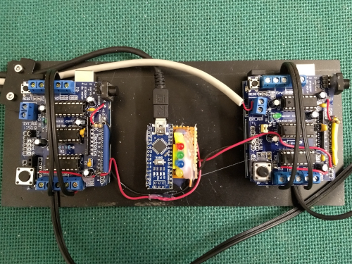
Figure 7. Arduinos used to control the food dispensers. The Jupyter notebook only communicates with the arduino nano in the middle of the picture by sending “on/off”-signals to different output channels of the microcontroller. Check out this post for the details.
Cell 6 initializes the micro-controller I use for controlling my food dispensers. In more detail, the cell activates communication with an arduino nano (Fig. 7, center position) and defines several output channels. Via two of these channels, the arduino nano can later send trigger pulses to two arduino unos with motor shields (Fig. 7, left and right position) controlling two independent feeders (Fig. 8). The three additional channels that are defined in cell 6 serve rather “cosmetic” purposes, as they are used to activate or deactivate a set of three diodes signalling different phases of the trial. In order to communicate with the arduino nano, you have to install the Firmata library to your micro controller. The arduino unos run a custom script, which you will also find in my GitHub repository.
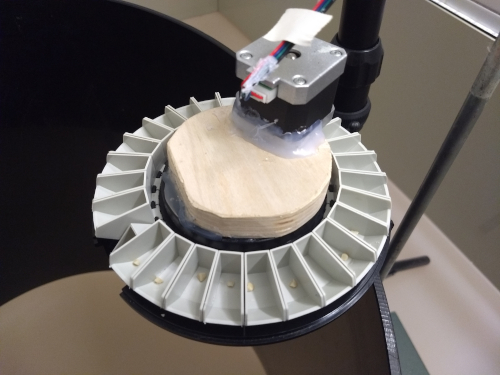
Figure 8. This is one of our DIY food dispensers. We used a commercially available fish feeder and added our own motor to it. The motor is connected to and controlled by one of the arduino unos from Fig. 7. The instructions on how to build these arduino controlled feeders will be covered in a future post
Cell 7 initializes the audio stream and loads the audio-files for later stimulation (Fig. 9). Please be aware that the sample .wav files I provide in my GitHub repository all have the same sound amplitude, but this does not mean that they will automatically be played back at the same volume by your setup. This, however, is vital for the experiment, as the idea is that the animals only use frequency information (and not volume information) for target detection. The volume or “loudness” of the stimuli will heavily depend on the properties of your audio hardware (sound card, cables, amplifier, loudspeaker). Therefore, before you even start your first experiment, you should thoroughly calibrate your audio stimulation using a high quality SPL meter. If you want to permanently adjust the amplitude of the sound files, you can do that in cell 7 by adding calibration factors to the code (Fig. 9).

Figure 9. Cell 7 initializes an audio stream and is used to load and calibrate the audio stimuli.
Taking a background picture
The tracking algorithm used by the script for real-time animal tracking compares every single frame of the video feed from our camera with a background image of the empty open field maze. This way the algorithm can easily detect any object that enters or leaves the arena. In a behavioral experiment, this should normally be the experimental animal and the droppings it leaves behind during the session. Since all of these objects are detected, the algorithm later chooses the largest of the detected objects as the experimental animal.
Before we can take the background picture for our current session, cell 8 generates an .avi container to which the video of our experiment will later be saved. You will find the video together with the other protocols in the same folder as the Jupyter notebook.
Execution of cell 9 starts the camera stream and opens a preview window that can be used to take the reference picture (Fig. 10). Make sure that the open field maze is clean and empty when taking the picture. Also, the illumination within the room should be the exact same as during your later experiments when you take it. If everything looks fine in the preview, press “c” on your keyboard to capture the background image. The image will automatically be saved and the window will close.
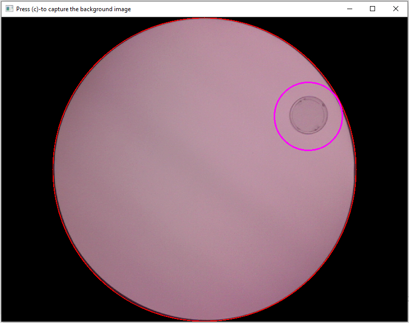
Figure 10. Use this window to capture the background image used for differential object tracking.
Final preparations
Now it is getting serious. Cell 10 opens another preview of the video feed. It looks highly similar to the preview from cell 9, but you can see a little more of the surroundings of your arena. You can use this preview for monitoring purposes during your final preparations. For example, you can double check if everything within the maze (e.g. the starting platform) is at its designated place. If you are happy with the maze and your final preparations, you can bring your experimental animal and put it into the arena. Needless to say, you should do this as careful as possible to avoid stressing the animal (for my mouse lemurs, I use a small, wooden box, in which the animals also sleep, for transportation and release them into the maze directly from this box). Afterwards, leave the room (I assume that your computer for monitoring and controlling the setup is in a different room than the arena itself) and observe your animal for at least a few more seconds to make sure that it is fine. If your experimental animal needs more time to accustom itself to new surroundings, you can also use this preview window to watch it a little longer while it habituates, before you start the experiment. As before, you can close the preview window pressing “c” on your keyboard.
Starting and stopping the experiment
Once the preview window has closed, you should run cells 11 to 14 in quick successions. Cell 11 initializes the final video stream for the video-based animal tracking. Cell 12 creates an .xlsx file to which the position of the animal and other task relevant information will be saved for each frame of the video stream. Cell 13 will open a pop up window with a start button (Fig. 11). This button mainly was included for users who run all cells at once instead of cell-by-cell to mark the point of no return. By hitting the button (or executing cell 14), the experiment starts and it will only stop, if the session time limit or the maximum trial limit is reached.

Figure 11. If you ran the Jupyter notebook using the “Run All” option from the “Cell” dropdown menu, clicking this button will start the experiment.
For monitoring purposes, you can watch the entire experiment in a live stream on your computer. If necessary for some unexpected reasons, you can also force the experiment to stop by pressing the “q” button on your keyboard. Never stop the script by simply closing the notebook or interrupting the kernel, as this will lead to data loss. Cell 14 has to shut down properly to save all the different protocol files.
Converting the protocol (optional)
Run cell 15, if you prefer .csv files over .xlsx files (as I certainly do). It will convert the Excel-based protocol of the experiment into a file with “comma separated values”.

Figure 12. If executed, cell 15 automatically converts the Excel-protocol from the experiment to comma seperated values for further processing in R.
After the experiment
The first thing to do after an experiment is over, is to catch the experimental animal and to bring it back to its home cage. Afterwards, I thoroughly clean the setup with 70% alcohol and immediately backup all relevant data from the experiment. On my backup drive, I have an individual folder for each experiment to which I copy the .txt file with the session parameters, the video of the experiment, and the .xlsx and/or .csv protocol. For analysis of the data, I usually work with the .csv file, as it can more readily be read and processed in R.
Additional notebooks
My GitHub repository for the sensory island task currently contains two additional Jupyter notebooks, “Two_Target_SIT.ipynb” and “Data Pre-processing.ipynb”. The former controls a SIT-variant with two target islands (“Two_Target_SIT.ipynb”; Video 2). The latter converts the .xlsx output from the experiments to MATLAB-files, which are used as input for the statistical analyses described in our methods paper.
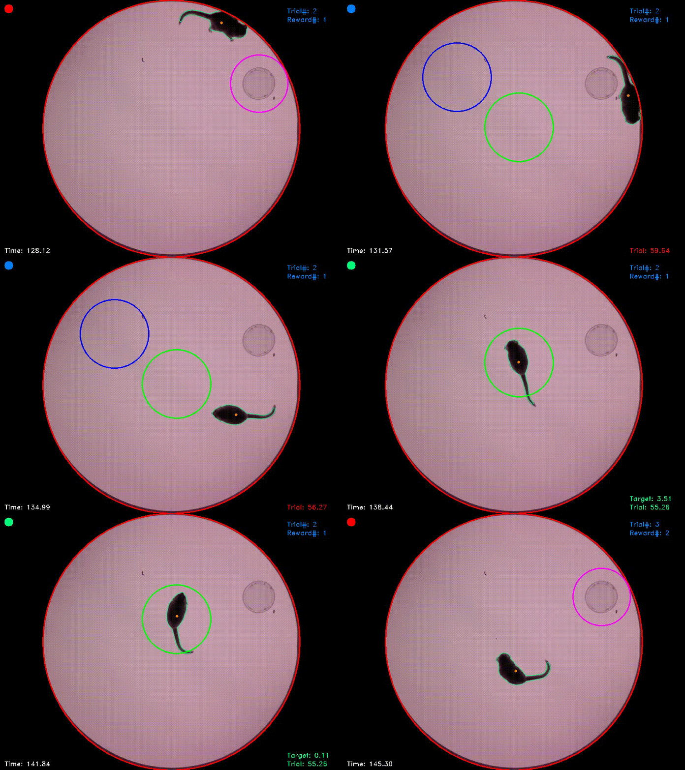
Video 2. In the experiment from which this video was taken, there were two target islands. As before, entering the green target triggered an acoustic attractor stimulus and staying in this area for the target duration was rewarded. Entering the blue target triggered a distractor stimulus and staying in this target had no consequences. As the reaction time was set to 1 second, the target areas in this experiment followed the animal’s position for this duration and were then fixed at their new positions. If the animal left a target area before trial completion, the area jumped back to its original position.